
Geometric Deep Learning on the Memecoin Graph
A memecoin's fate lives in a graph of creators, tokens and wallets — not a price series. A geometric-deep-learning study that proves the relational reframe is right, shows that graph topology does not beat a DeepSets ‘bag of wallets’, proves why the naive spectral operators degenerate on single-token star ego-graphs, and isolates the one non-price signal that survives: cross-token wallet convergence.
In brief
A rigorous, adversarially-audited geometric-deep-learning study of whether a memecoin's fate is learnable from the relational graph of creators, tokens and wallets rather than from its price series. The reframe is intellectually right and empirically unproven: under matched controls, graph topology does not beat a DeepSets ‘bag of wallets’ (ΔAP −0.011 at $1M), the learned GNN never beats a logistic baseline, the headline AUCs are a source confound (pooled 0.97 → ~0.76 within one source), and the deployed model sits on a zero-parameter volatility null. The paper proves why the naive spectral operators degenerate on single-token star ego-graphs, and isolates the one real non-price signal — cross-token wallet convergence (coordination), ~237× denser than chance — together with its strict scope limits.
Key results
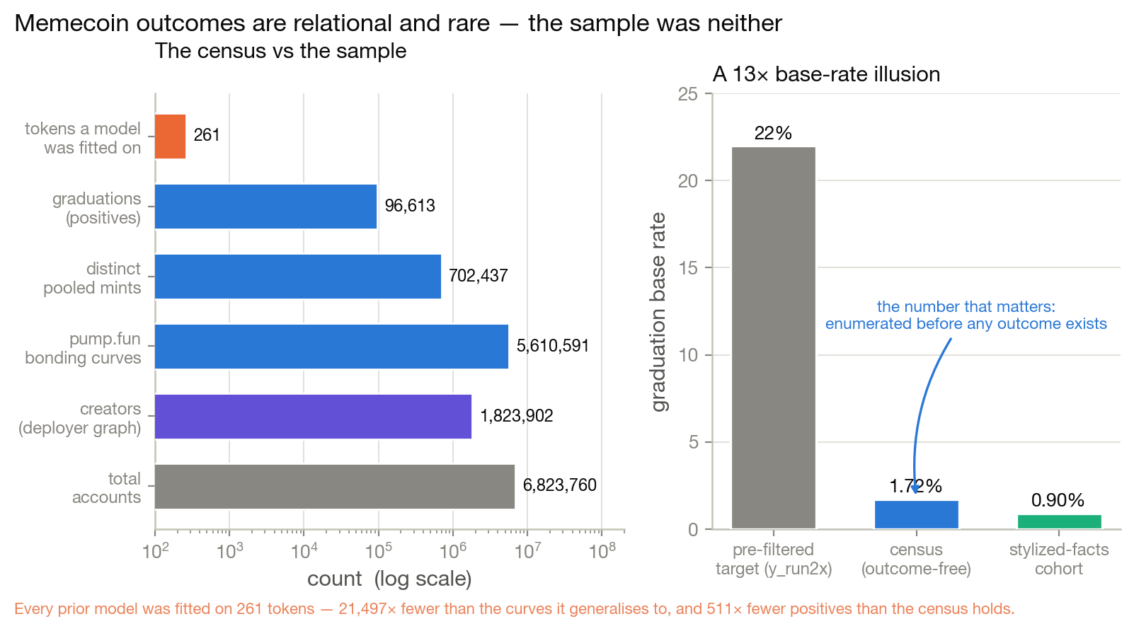
- An outcome-independent Solana census settles the base-rate illusion: across 5,610,591 pump.fun bonding curves exactly 96,613 graduate — a 1.72% rate measured before any outcome exists — against the ~22% pre-filtered event every prior model trained on, over a deployer graph of 1,823,902 creators and 6,823,760 accounts (prior models were fit on 261 tokens).
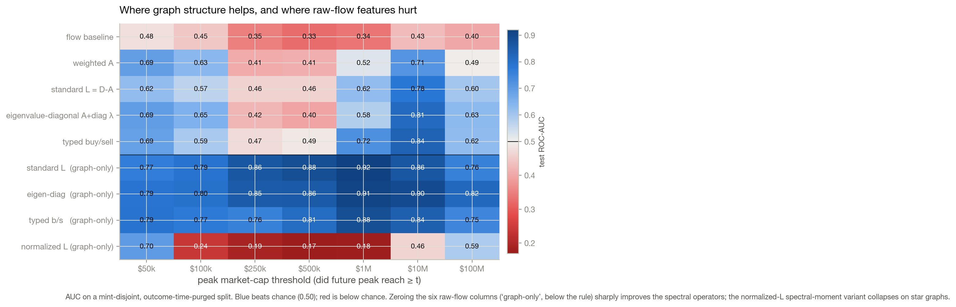
- Graph structure helps only after the raw-flow columns are deleted: on a mint-disjoint, outcome-time-purged split, 'graph-only' spectral operators reach test ROC-AUC 0.86–0.92 on the mid-cap heads while the flow baseline sits below chance at 0.33–0.48; the normalized Laplacian collapses to 0.17–0.24, exactly the star-graph degeneracy.
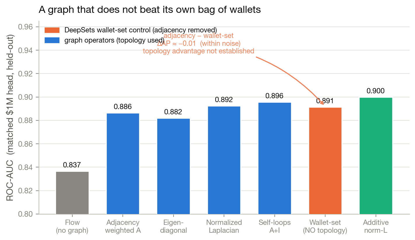
- The topology control: a matched DeepSets 'wallet-set' encoder, handed the same wallets with the adjacency removed, ties the graph — paired adjacency−set ΔAP = −0.011 [−0.028, +0.001] at the $1M head. The pilot does not establish that topology adds anything beyond the bag of wallets.
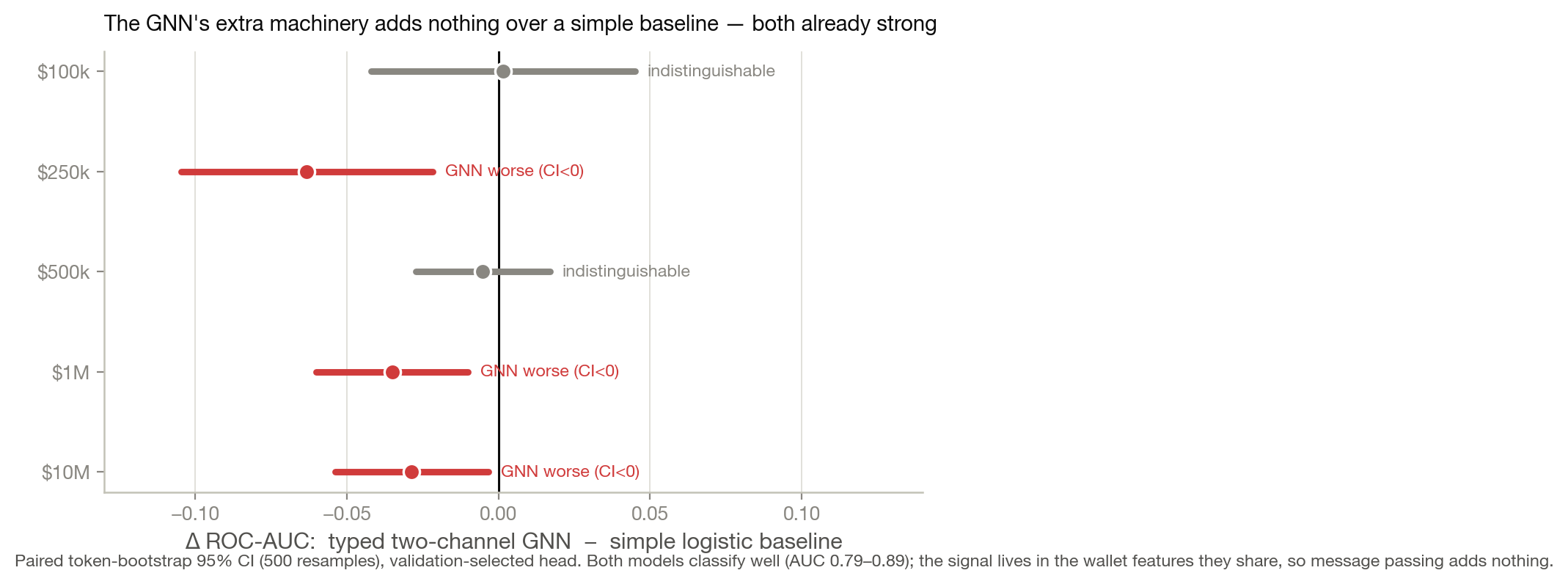
- The typed two-channel GNN classifies well (test ROC-AUC 0.79–0.89 across all fourteen heads; log-peak regression test R² 0.61–0.73) but does not improve on a plain logistic over the same wallet features — paired ΔROC-AUC [−0.105, −0.022] at $250k, [−0.060, −0.010] at $1M. On single-token stars there is simply no extra structure for message passing to exploit; the network is verifiably permutation-equivariant.
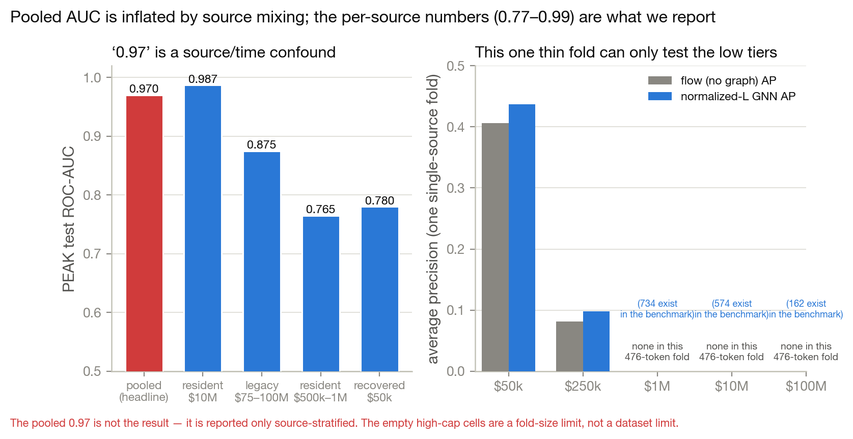
- The pooled AUC is partly a source/time confound: 0.97 is reported only source-stratified (resident-$10M 0.987, resident-$500k–$1M 0.76–0.77), and the empty high-cap cells on one 476-token single-source fold are a fold-size limit — not a dataset limit: the benchmark itself holds 734 / 574 / 162 positives at $1M / $10M / $100M.
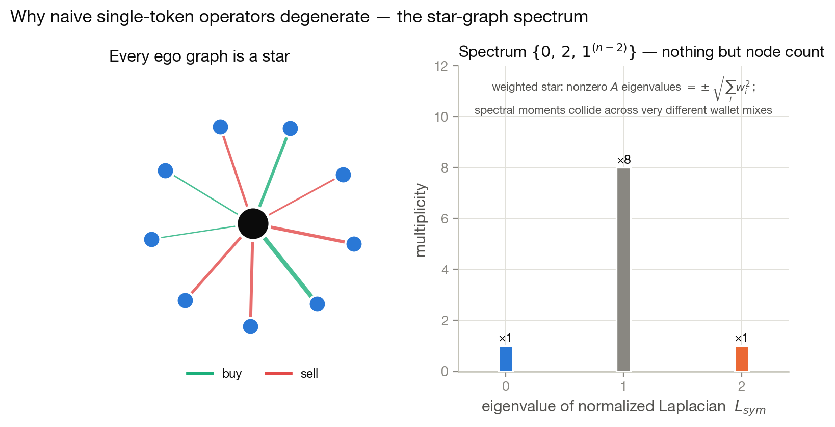
- Two proofs of why the naive operators fail: every single-token ego graph is a star, so its weighted adjacency has only the nonzero eigenvalues ±√(Σwᵢ²) and its normalized-Laplacian spectrum is {0, 2, 1^(n−2)} — spectral moments re-encode node count; and the eigenvalue-diagonal operator A+diag(λ) is not permutation-equivariant (measured error up to 7.43 vs ~1e-14 for the Laplacians).
- The deployed model (AUC 0.759) sits on a zero-parameter Brownian-volatility null (0.757); a 103-column single-feature sweep beats the null 0 times, a 336-cell cost-aware backtest has 0 cells with P&L above zero, and moonshots (≥31.6×) score AUC 0.444. The one non-price signal that survives is cross-token wallet convergence — survivors vs collapses separate with Cliff's δ ≈ 0.65–0.70, coordinated buyer clusters ~237× denser than chance — but only within one source and only forward-looking.
The Whole Memecoin Graph in One Frame
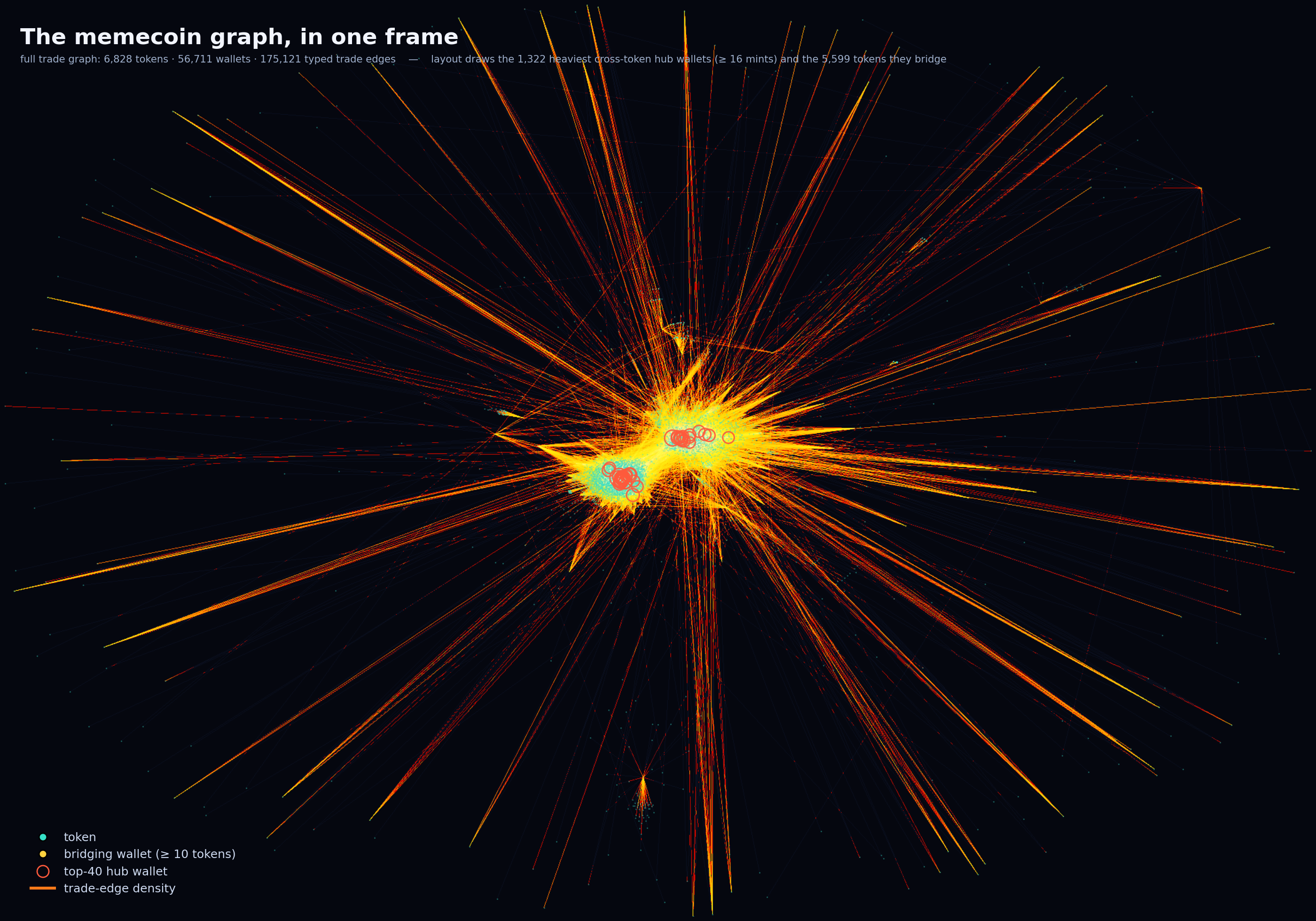
Before any model, here is the object itself. We assembled the bipartite wallet–token trade graph from every committed panel snapshot — 6,828 tokens, 56,711 wallets and 175,121 typed trade edges, roughly 1.9M SOL of flow — and rendered it in a single Datashader frame, edges shaded by a histogram-equalised count so density reads directly. Tokens are teal; the wallets that traded them surround them; trade-edge density is the glow.
To keep the layout legible we draw only the cross-token wallets — the tens of thousands that touched more than one mint — and omit the single-token leaf halo. What the picture makes immediate is the thing the rest of the paper spends twenty pages quantifying: a small set of wallets recurs across a great many otherwise-independent tokens. One wallet alone touches 3,026 distinct mints; 2,766 wallets touch ten or more. These are the bright hubs that stitch unrelated tokens into shared components.
That recurrence — not any per-token wiring — is the signal that survives every control later in the paper. The graph shows it before a single parameter is fit: coordination is visible as topology, as hubs, long before it is visible as a number.
Two Illusions About Predicting a Memecoin
The dominant way to ask 'can you predict a memecoin' is tabular: each token is an independent row of hand-crafted scalars — early volume, holder counts, buy/sell ratios — and a classifier is fit to a binary label like hit_1M. That framing hides two illusions, and this paper starts by dismantling both.
The first is a sampling illusion. A market-cap-sorted census of 'tokens that reached a pool' implies a graduation rate near 52%; a cohort selected on early features plus a realized outcome — never on the outcome — puts the true rate at 4.2%, falling to 0.95% across a 1.25M-token population as pump.fun saturated. Enumerating the chain directly settles it: across 5,610,591 pump.fun bonding curves, exactly 96,613 graduate — a base rate of 1.72%, measured before any outcome exists. Every model in the predecessor program targeted a pre-filtered ~22% event, an order of magnitude away from the population it must generalize to.
The second is an i.i.d. illusion. Those same models were fitted on 261 tokens. The census holds 21,497× as many curves and 511× as many positives — and it is not a bag of rows but a deployer graph over 1,823,902 creators and 6,823,760 accounts. Aggregating that graph to scalars is a lossy projection: the established finding that concentration beats breadth (a tightly held token outruns a broadly held one, univariate AUC 0.92 inverted) is itself a shadow of a graph property measured through a scalar proxy.
What the Raw Data Already Dictates
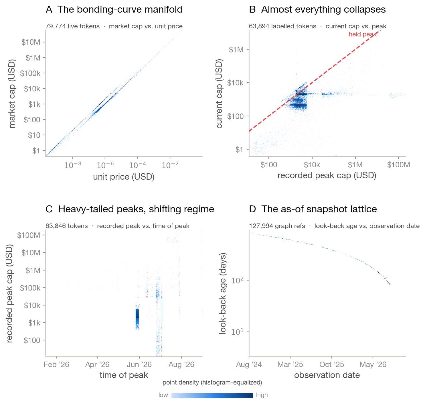
Before a single model is fit, four pictures of the committed recovery data — rendered directly with Datashader, no sampling — fix the constraints the rest of the paper has to respect. The program itself spans three nested scales that we keep rigorously apart: a census of 5,610,591 bonding curves (no model is trained on it), tabular graduation models trained on hundreds of thousands of tokens that predict well out of time (714,747 early-window, launch-time GBM ROC 0.95; 1,024,000 recent, up to deep-MLP 0.99; over 613k creators), and the graph benchmark of 10,344 mint-disjoint snapshots over 5,172 mints (test fold 2,204) on which every GNN result here is measured. The panels below are plotted from the real recovery tables: 79,774 live tokens, 63,894 labelled tokens and 127,994 graph references.
First, every live token sits on a near-deterministic market-cap–price manifold (panel A): unit price is almost a fixed function of reserves, so a 'price' feature is largely a restatement of market cap and carries little independent information. Second, measured against their own recorded peak, almost all tokens have already collapsed (panel B): the mass of points sits far below the held-peak diagonal, pinned to a sub-$10k floor — the drawdown that any realistic study has to treat as the base case.
Third, the surviving peaks are heavy-tailed and regime-shifting (panel C), spanning five orders of magnitude and clustering into discrete collection batches rather than a stationary stream. Fourth, the labels themselves form an as-of lattice (panel D): each token is observed at a fixed calendar date looking back a fixed horizon, and that geometry is exactly what turns a careless snapshot join into a leak of the future. Every downstream choice — token-level splits, outcome-time purging, the gsnap_ discipline — is a response to one of these four facts.
These are not schematic illustrations; they are the raw distributions, and the rarity, the collapse and the as-of structure they show are why the measured numbers later in the paper fall so far below the pooled headline.
A Memecoin Is a Graph, Not a Price Series
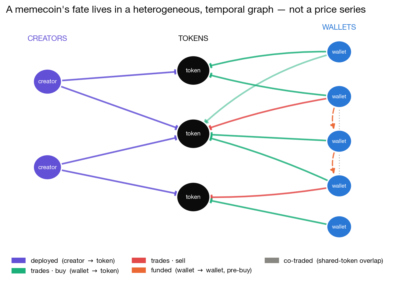
We take the relational object seriously. A creator deploys tokens; a token is a mint; a wallet trades tokens; an event (wallet, token, time) is a timestamped trade, the unit of prediction. Edges come in four relation types: deployed (creator → token), trades (wallet → token, signed buy/sell), funded (wallet → wallet, a native-token transfer before the recipient's first buy — the seeding signature of a non-organic launch), and co-traded (shared-token overlap). The coordination that actually moves these markets lives in those wallet–wallet edges, where no price feature can see it.
The central question the whole program exists to test is simple: when several wallets buy the same token, are they independent actors (organic discovery) or a connected cluster (coordination)? A token bought by eight wallets that all fund or follow each other is a different object from one bought by eight strangers — and market-cap features cannot tell them apart.
The discipline here is mostly about time. The follow graph is a single present-day snapshot; it contains edges created after historical trades, so joining it onto past events leaks the future. Every such column carries a gsnap_ prefix to make the hazard impossible to forget: these quantities are valid for forward-looking scoring, never for a backtest. And because the intra-token correlation is high (ICC 0.638, design effect 46.7), we train and evaluate at the token level, with mint-disjoint, out-of-time splits and token-clustered bootstraps throughout.
The Ego Graph as the Unit of Computation
The full heterogeneous graph is never materialized. Every model instead reads a bounded ego graph centered on one token, because scoring has to be inductive and per-token — a fresh mint must be scored from its own neighborhood, with no retraining — and the serve-time budget is fixed. Two ego constructions do two different jobs.
The training ego graph is a star on 24 nodes (CAP=24): the token as node 0 and its top 23 wallets by known-prefix SOL volume. Each observed trade adds a weight log(1+SOL)+0.1 into one of two typed, symmetrically normalized adjacencies (buy, sell); no wallet–wallet edge is ever fabricated. Each node carries 14 features — four flow measures (buy count, sell count, buy SOL, sell SOL), each kept as a level, a trailing-60s rate and a difference-of-rates acceleration, plus two node-type indicators — and a panel of global graph summaries (buyers, sellers, buy-wallet HHI and top-1 share, shared-wallet and neighbor-token counts, bipartite four-cycles, signed SOL/USD flow) is concatenated at readout. This is the exact object fed to the typed GNN and its wallet-set ablation.
The deployed system exposes a second, larger ego view — _ego(mint, radius_buyers=50): the token's top 50 wallets by SOL size, each annotated with its token degree (how many of our tracked tokens the wallet also trades) and a pairwise co-trade overlap. This one is deliberately a descriptive view, not a classifier: a high token degree flags shared activity for a human analyst, and the code says in as many words that it is not proof of a common controller. It is how the coordination hypothesis is triaged live, and it is where the surviving convergence signal is read off.
The ego graph is the right unit — local, inductive, cheap — and it is also the origin of the degeneracy proved next. A single-token ego graph with no fabricated edges is a star; and ranking wallets by SOL and keeping the top 23 discards the long tail, so a token with 25 buyers and one with 2,500 can present the same selected neighborhood. The construction that makes scoring tractable is the same one that caps what a purely spectral reading can see — which is precisely why the specified frontier model replaces the single-token star with a bounded 2-hop, multi-token neighborhood.
The Outcome Is Learnable
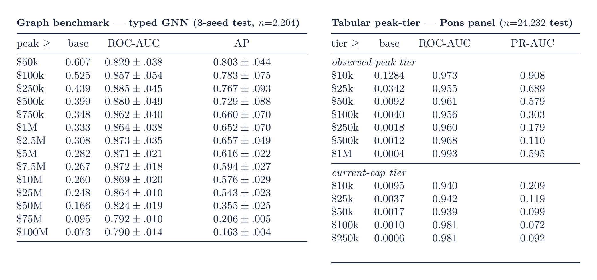
Before the controls, the plain fact: the target is learnable, and the models fit it well — at every scale, including the largest. The tabular graduation family, trained on hundreds of thousands of tokens, predicts graduation strongly out of time: the deployed early-window model reaches gradient-boosting ROC 0.95 with 23× top-1% lift on 714,747 tokens, and on the 1,024,000-token recent store a logistic 0.95 rises through GBM 0.98 to a deep MLP at 0.99 (11×→41× lift). These are large, out-of-time, leakage-controlled results — not a thin pilot.
On the graph side the typed two-channel GNN reaches test ROC-AUC 0.79–0.89 across all fourteen nested peak heads on the mint-disjoint, three-seed split ($50k 0.829, $250k 0.885, $1M 0.864, $100M 0.790), and the Pons peak-tier panel (n = 24,232 test) reaches ROC-AUC 0.955–0.993 on observed-peak tiers and 0.94–0.98 on current-cap tiers — precision concentrated in exactly the top percentile a scout would inspect. The out-of-time learnability bake-off agrees: hist-GBM hits ROC 0.906 / 0.928 / 0.912 on the hit_250k / hit_500k / hit_1M heads.
That these targets are learnable is not the claim this paper contests. The controls that follow ask the two harder questions — what the signal is attributable to (the wallet set, not its wiring) and whether the specifically geometric gains survive source and time shift — and those are where the geometric story narrows. Read these numbers as the ceiling the rest of the paper interrogates.
The Operator Zoo, and Where Structure Helps
On a bounded bipartite ego graph — the token as node 0, its top wallets as leaves, no invented wallet–wallet edges — we build an operator zoo: the combinatorial Laplacian L = D − A, the symmetric-normalized Laplacian L_sym = I − D^(−1/2) A D^(−1/2), a GCN renormalization, typed buy/sell channels, and the lab's signature eigenvalue-diagonal operator B = A + diag(λ), the adjacency with the graph's own eigenvalues written onto its diagonal. Each operator is either compressed to eight spectral moments and fed to a logistic/ridge model, or used as the propagation matrix of a typed two-channel message-passing GNN.
The learnability map holds a surprise. The raw-flow baseline is at or below chance (0.33–0.48) on the mint-disjoint split: the six flow columns a tabular model would lean on do not survive source/era shift. Zeroing those columns ('graph-only') sharply improves the spectral operators — standard_L climbs to 0.86–0.92 on the mid-caps — while the normalized Laplacian collapses to 0.17–0.24. Structure helps, but only once the actively harmful flow features are removed, and only for the operators the degeneracy spares.
That collapse is not noise. It is the signature of a specific, provable failure mode, which the next section makes precise.
Why the Naive Operators Cannot Work
A single-token ego graph with no invented wallet–wallet edges is a star: one hub (the token) joined to n−1 leaves (wallets), and nothing else. Stars are spectrally almost empty. A weighted star's adjacency has rank 2, so zero is an eigenvalue of multiplicity n−2; since the trace is zero the two remaining eigenvalues are ±μ, and the trace of A² pins μ = √(Σ wᵢ²). For an unweighted star the normalized-Laplacian spectrum is exactly {0, 2, 1^(n−2)}.
The consequence is a corollary that kills the method: the eight spectral moments of L_sym on an ego-star are a function of node count alone, and of A a function of (node count, weight energy) alone. Two ego graphs with the same number of wallets and the same weight energy but entirely different trading behaviour collide before the learner receives them. This is not a worst case — it is the typical case, because every ego graph in the corpus is a star. It predicts exactly the normalized-L collapse in the heatmap above.
The eigenvalue-diagonal operator fails for a second, independent reason: it is not permutation-equivariant. Writing eigenvalues onto the diagonal under an index-order assignment makes the model's output depend on wallet ordering — an artifact with no market meaning. Measured on held-out ego graphs, its operator-equivariance error is as large as 7.43 against ~1e-14 for the Laplacians, so we refuse to rank it as a winner wherever it appears to lead.
A Graph That Does Not Beat Its Own Bag of Wallets
A graph model that beats a flow baseline has proven only that wallets carry signal, not that their wiring does. The correct control is a DeepSets wallet-set encoder: the same multiset of wallets with the same features, but the adjacency replaced by the identity — topology removed. The question 'does the graph add anything beyond the bag of wallets?' is exactly this control versus the full GNN.
On a matched $1M comparison (same split, seed and 8-node budget), topology and set are a dead heat. The paired adjacency−wallet-set advantage is ΔAP = −0.011, with a 95% interval of [−0.028, +0.001] that straddles zero. We therefore state plainly that this pilot does not establish a topology advantage; the apparent graph-versus-flow gap conflates input set, model family and node budget, and once those are matched the wiring earns nothing.
This is the paper's central negative result, and it is the kind the field rarely runs: not graph-versus-tabular, but graph-versus-its-own-contents.
The Learned GNN Never Wins the Paired Test
The typed two-channel GNN classifies well — the same 0.79–0.89 AUCs above. The narrower question is whether its message passing adds anything over a plain logistic regression on the same wallet features. Validation-selected per head and compared by a token-paired bootstrap, its ΔROC-AUC against the logistic is either indistinguishable from zero or mildly negative at every threshold: [−0.105, −0.022] at $250k, [−0.060, −0.010] at $1M, [−0.054, −0.003] at $10M. On the continuous target the GNN is, by contrast, a solid regressor — test log-peak R² 0.61–0.73 on the benchmark (it collapses only on a tiny 10-token end-to-end prefix). The extra machinery simply does not need the adjacency a bag-of-wallets model lacks.
The failure is not a bug. Node-permutation outputs match to ~1e-8, confirming the network is genuinely equivariant — it is a faithful graph model, and it still does not beat a logistic regression on the same inputs. On single-token star neighborhoods, there is simply not enough structure for message passing to exploit beyond what a set encoder or a linear model already extracts.
The Source Confound, the Free Rule, and the Brownian Null
The headline that makes memecoin graph-learning look solved — pooled AUC ~0.97 — is a source/time artifact. Reported source-stratified, the same models give resident-$10M 0.987 but resident-$500k–$1M only 0.76–0.77; on one 476-token single-source trajectory fold the average precision barely clears prevalence. The $1M/$10M/$100M heads are empty on that one fold — a fold-size limit, not a dataset limit: the benchmark itself holds 734 / 574 / 162 positives at those tiers. Part of the pooled headline lives in the mixing of a legacy ATH-labelled source with a resident-trajectory source, not purely in the graph.
The deployer graph fares no better against a free baseline. Folding a nine-feature deployer block into nine market-cap tier heads over 1.33M rows and 65,138 tokens, and scoring 'hits per 15 tokens inspected' against the free market-cap-sort rule, the learned head wins only at the bottom: +0.14 at $100k and +0.05 at $250k, but −0.04 at $1M, −0.11 at $5M and −0.09 at $10M. Above $250k, sorting by one column you already have beats the model. (A commit message claimed the deployer block 'improves $500k/$1M/$5M and hurts none'; the committed numbers contradict it, and we report the numbers.)
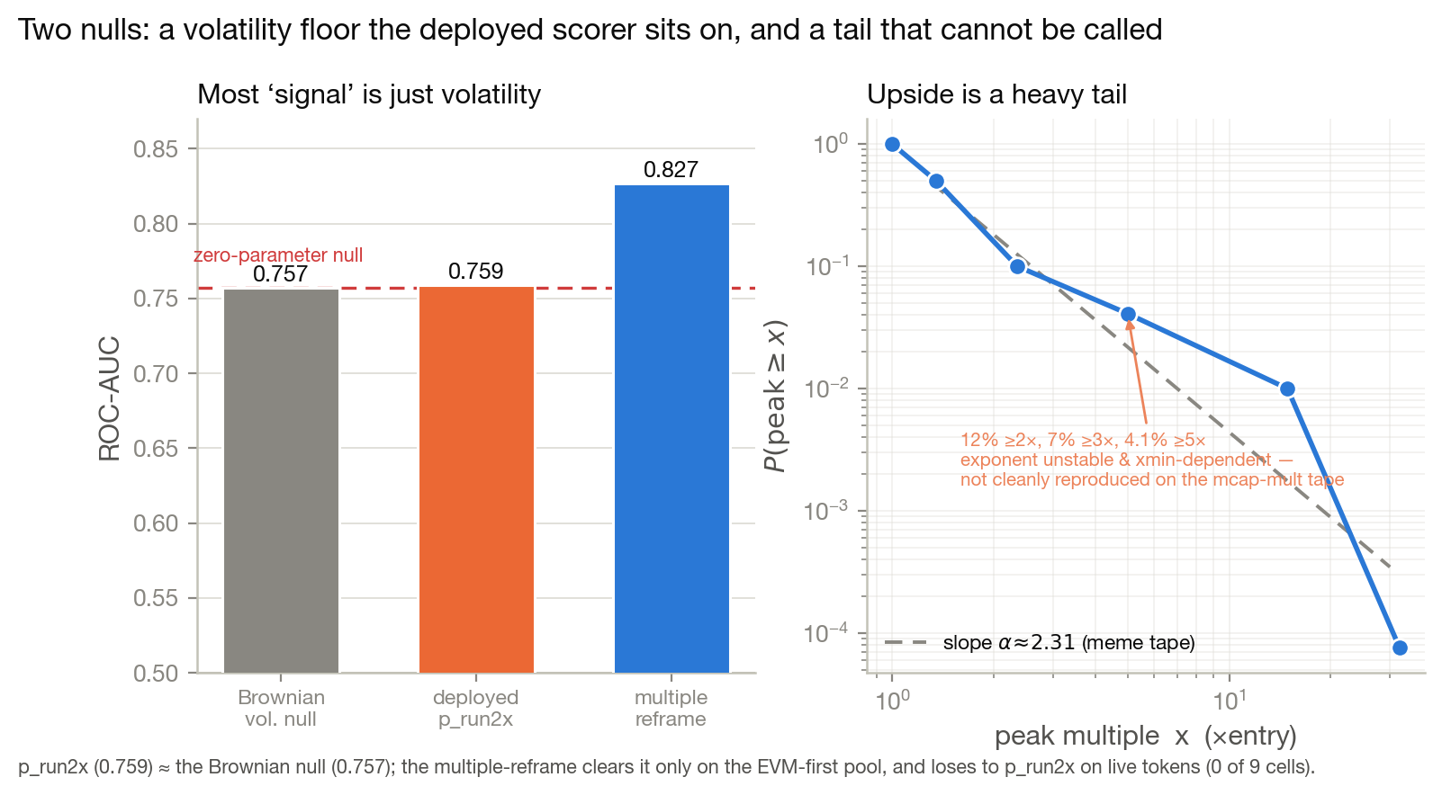
Worse still, the deployed production scorer (AUC 0.759, top-5% lift 2.53×) is statistically indistinguishable from a zero-parameter Brownian-volatility null (0.757): much of the apparent signal is just 'volatile things move more.' A 103-column single-feature sweep beats the null 0 times; a 336-cell cost-aware backtest has 0 cells with P&L confidence above zero; moonshots (≥31.6×, ≥100×) score AUC 0.444 and 0.407 — below a coin flip. The leakage-free ceiling is ≈0.76 AUC once a lifetime-count leak is removed.
The One Signal That Survives
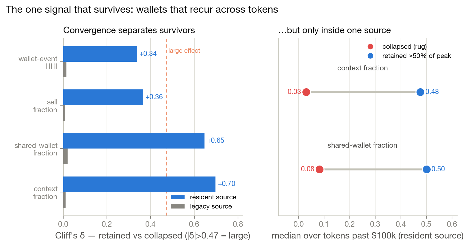
Strip away everything that fails a control, and one structural phenomenon remains — and it is exactly the coordination the program was built to find. Among tokens past $100k on the resident source, survivors (retained ≥50% of peak) and collapses (rugged to <10%) separate with large Cliff's δ on precisely the cross-token quantities: +0.70 on context fraction, +0.65 on shared-wallet fraction, +0.37 on sell fraction and wallet-event concentration. At the population level, 65% of tokens are bought by an all-islands set of mutually unconnected wallets, while the 35% carrying any follow edge have a buyer subgraph ~237× denser than the ambient graph — a self-pump signature that is invisible to every price feature.
The mechanism is coherent: buys are self-exciting (a Hawkes branching ratio approaching 1 marks a token going critical), and concentration beats breadth because a high top-buyer share raises both the effective coordination of the beauty contest and the persistence of informed order flow. This is the non-price edge, and it is real.
But it is narrow, and we say so twice. The separation is source-conditional: on the legacy source the same Cliff's δ is ≈ +0.01, no separation at all. And the 237× and the convergence features are present-day snapshot (gsnap_) quantities — valid for forward-looking scoring, never as backtest inputs. The signal is genuine, non-price, and strictly scoped.
Verdict
The geometric reframe is intellectually correct and empirically unproven. Under matched controls, topology does not beat a bag of wallets; the learned GNN does not beat a logistic regression; the strong AUCs are a source confound; the deployed model sits on a zero-parameter volatility null; and the signature eigenvalue-diagonal operator is not even equivariant. What is real is small: a thin, locatable edge at $100k–$250k, a genuinely non-price coordination signal with a large within-source effect, and a precise account of why the naive operators degenerate.
Three limitations are structural, not incidental. The graph is not yet built — the funded graph has 0 collected rows, and only 2 of 104 buy events carry a full one-hour forward window, so the frontier heterogeneous temporal GNN is specified but unbuildable until the firehose backfill lands. The ego graph is a star — until multi-token, multi-hop neighborhoods replace single-token stars, the spectral degeneracy caps what any spectral method can see. And the economics are tail-driven — a cost-aware entry into the top decile returns +11.1% per trade at 3% cost but wins only 28–38% of the time with a median trade of −2% to −7%. This is not a money printer; a prior shipped $1M head was found degenerate against fixture-fabricated base rates. The deliverable is not an edge but a reproducible map of where the edge is and is not — and a clear statement of the data and multi-hop structure that would be needed before geometric deep learning on memecoin markets could clear its own nulls.
Abstract
A memecoin is usually modeled as a price series: a token is a row, its features are scalars, and a classifier predicts whether it will ‘moon.’ We argue the data is relational, not i.i.d. — creators launch many tokens, wallets trade many tokens, and the coordination that actually moves these markets (bot fleets, shared funding sources, self-pump rings) lives in the graph, not in any per-token row. This is a geometric-deep-learning study of that claim, built from two code bases (GACWR/fomo, GACWR/meme-research) at three nested scales kept rigorously apart: an outcome-independent Solana census of 5,610,591 bonding curves, 1,823,902 creators and a 1.72% graduation base rate; tabular graduation models trained on hundreds of thousands of tokens that predict well out of time (714,747 early-window tokens, launch-time gradient boosting ROC 0.95 with 23× top-1% lift; 1,024,000 recent tokens, logistic 0.95 → GBM 0.98 → deep-MLP 0.99, 11×→41× lift); and the graph benchmark on which the specifically geometric claim is tested — 10,344 mint-disjoint snapshots over 5,172 mints (test fold 2,204). We formalize a heterogeneous, temporal wallet–token–creator graph; build an operator zoo (combinatorial and symmetric-normalized Laplacians, a GCN renormalization, a signature eigenvalue-diagonal operator, and typed buy/sell channels); and train a 1-hop creator prior, spectral-moment logistic models, and a typed two-channel message-passing GNN, each under strict mint-disjoint, outcome-time-purged, token-clustered validation. Both model families fit the target well; the audit is deliberately strict about what that signal is attributable to, and it narrows the specifically geometric claim. Graph structure helps only after the raw flow columns are removed — ‘graph-only’ spectral operators reach test ROC-AUC 0.86–0.92 on the mid-cap heads while the flow baseline sits below chance (0.33–0.48) — yet against a matched DeepSets ‘wallet-set’ control handed the same wallets with no adjacency, the paired topology advantage is within noise (ΔAP ≈ −0.01 at the $1M head): a graph that does not beat its own bag of wallets. The typed GNN classifies well (ROC-AUC 0.79–0.89 across all fourteen heads; test log-peak regression R² 0.61–0.73) but does not improve on a logistic regression over the same wallet features — on single-token stars there is no extra structure for message passing to exploit. The pooled 0.97 is partly a source/time confound — within a single source AUCs run 0.76–0.99 — and the empty high-cap cells on one 476-token trajectory fold are a fold-size limit, not a dataset limit (the benchmark holds 734/574/162 positives at $1M/$10M/$100M). On the client's own market-cap tiers a deployer-graph head beats the free market-cap-sort rule only at $100k/$250k, and the deployed model (AUC 0.759) is statistically indistinguishable from a zero-parameter Brownian-volatility null (0.757). We also prove why the naive single-token operators degenerate: every ego graph is a star, whose weighted adjacency has only the two nonzero eigenvalues ±√(Σ wᵢ²) and whose normalized-Laplacian spectrum is {0, 2, 1^(n−2)}, so spectral moments mostly re-encode node count; and the eigenvalue-diagonal operator is measurably not permutation-equivariant. The one durable, genuinely non-price signal is cross-token wallet convergence: survivors and collapses separate with large Cliff's δ on shared-wallet and context fractions, and coordinated buyer clusters are ~237× denser than chance — but only inside a single source and only as a forward-looking snapshot quantity, never a backtest feature. The deliverables are the validated predictive models and this surviving signal, together with a first-class catalogue of the leakage traps, nulls and degeneracies that bound them.
More figures
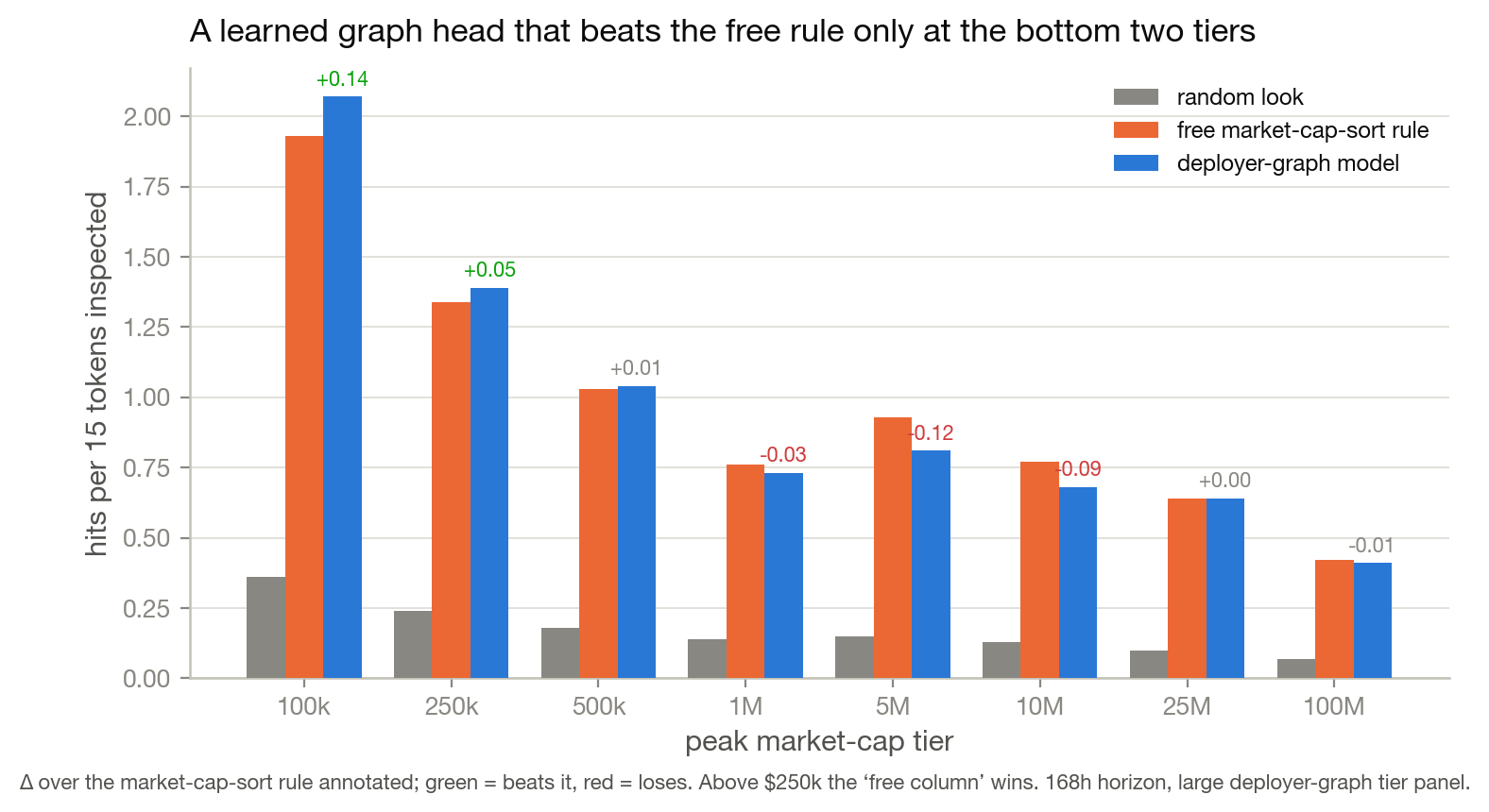
Fig. 1A deployer-graph tier head versus the free market-cap-sort rule (and a random look), scored as hits per 15 tokens inspected over 1.33M rows / 65,138 tokens. The learned head beats the free rule only at $100k (+0.14) and $250k (+0.05); above $250k, sorting by one column you already have wins.